


.
O P E N A C C E S S S O U R C E : AgING
Abstract
Aging has pronounced effects on blood laboratory biomarkers used in the clinic. Prior studies have largely investigated one biomarker or population at a time, limiting a comprehensive view of biomarker variation and aging across different populations. Here we develop a supervised machine learning approach to study aging using 356 blood biomarkers measured in 67,563 individuals across diverse populations. Our model predicts age with a mean absolute error (MAE), or average magnitude of prediction errors, in held-out data of 4.76 years and an R2 value of 0.92. Age prediction was highly accurate for the pediatric cohort (MAE = 0.87, R2 = 0.94) but inaccurate for ages 65+ (MAE = 4.30, R2 = 0.25). Variability was observed in which biomarkers carry predictive power across age groups, genders, and race/ethnicity groups, and novel candidate biomarkers of aging were identified for specific age ranges (e.g. Vitamin E, ages 18-44). We show that predictors for one age group may fail to generalize to other groups and investigate non-linearity in biomarkers near adulthood. As populations worldwide undergo major demographic changes, it is increasingly important to catalogue biomarker variation across age groups and discover new biomarkers to distinguish chronological and biological aging.
Introduction
Aging has pronounced effects on blood laboratory biomarkers used in the clinic such as testosterone [1] and plasma fibrinogen [2]. As worldwide populations undergo major demographic and aging shifts [3], it will be increasingly important to understand how aging relates to not just single blood biomarkers but combinations of many blood biomarkers together, particularly for age-associated diseases that lack inexpensive and noninvasive tools for early detection and staging such as Alzheimer’s disease [4]. Studies of laboratory analytes and aging have traditionally considered a single analyte at a time [5–7] and have been limited in their inclusion of demographically diverse groups [8]. Simultaneously modeling many blood biomarkers together across population groups paints a more complete picture of health and disease and enables the systematic study of differences resulting from the definitions of age based on time since birth (“chronological age”) and as a cumulative measure of biological wear and tear (“biological age”) [9].
Recently, machine learning and statistical methods have enabled agnostic, data-driven approaches to age prediction based on methylation [10, 11], transcriptomic [12], and retinal imaging data [13]. For example, in 2018, researchers at Google used deep neural networks to analyze retinal fundus images to predict cardiovascular risk factors including a patient’s age [13]. While machine learning has been widely applied to fields such as medical imaging [14, 15] and speech recognition [16, 17], it is comparatively underapplied in the study of blood laboratory biomarkers [18, 19], which may be among the cheapest to measure in individuals.
In this study, we apply supervised machine learning methods to 356 blood laboratory measures from 67,563 individuals. Our aim is to systematically study the predictive capacity of individual and large collections of blood laboratory biomarkers for predicting chronological age across the lifespan. We compute aging curves for all blood laboratory measures and assess whether changes in the predictive power of individual biomarkers are consistent across different populations with respect to gender, race, and income. We document how age predictors that perform highly accurately in one population may generalize poorly to different populations and use piecewise linear regression methods to investigate significant age-related changes in the trajectories of laboratory analytes. Our results identify clear demographic structure embedded in blood laboratory data and show that we are able to predict chronological age from laboratory analytes with high accuracy, which compares favorably to top predictors in the field [20].
Results
Age is highly predictable from blood laboratory analytes
We trained a random forest model [21] to predict chronological age (in years) using data from 67,563 individuals ranging in age from 1 to 85 years (mean: 36.2, standard deviation: 23.1) from nine CDC National Health and Nutrition Examination Survey (NHANES) cohorts spanning 1999-2016 (Figure 1), a representative sample of the non-institutionalized population of the United States. The model included 356 features consisting of laboratory analytes (e.g. serum glucose, creatinine). Many of the analytes contained a large proportion of missing data (Supplementary Table 3), which was dealt with by imputing missing values using mean imputation. We evaluated model performance both using five-fold cross-validation and held-out data (Methods). Hyperparameters were selected by grid search (Methods). We define our baseline model for chronological age prediction as a linear regression model without regularization, using age as the response variable and the 356 laboratory analytes as covariates. Mean absolute error (MAE) for the baseline linear regression model was 10.53 (SE: 0.07) years in five-fold cross-validation and 10.52 years in the 20% held-out dataset. The R2 for the baseline model was 0.63 (SE: 0.01) in the five-fold cross-validation and 0.62 in the held-out set. In our best random forest model, MAE was 4.80 (SE: 0.013) years in cross-validation and 4.76 years in the 20% held- out dataset. The R2 from the random forest model was 0.92 (SE: 0.0005) in the five-fold cross-validation and 0.92 in the held-out set.
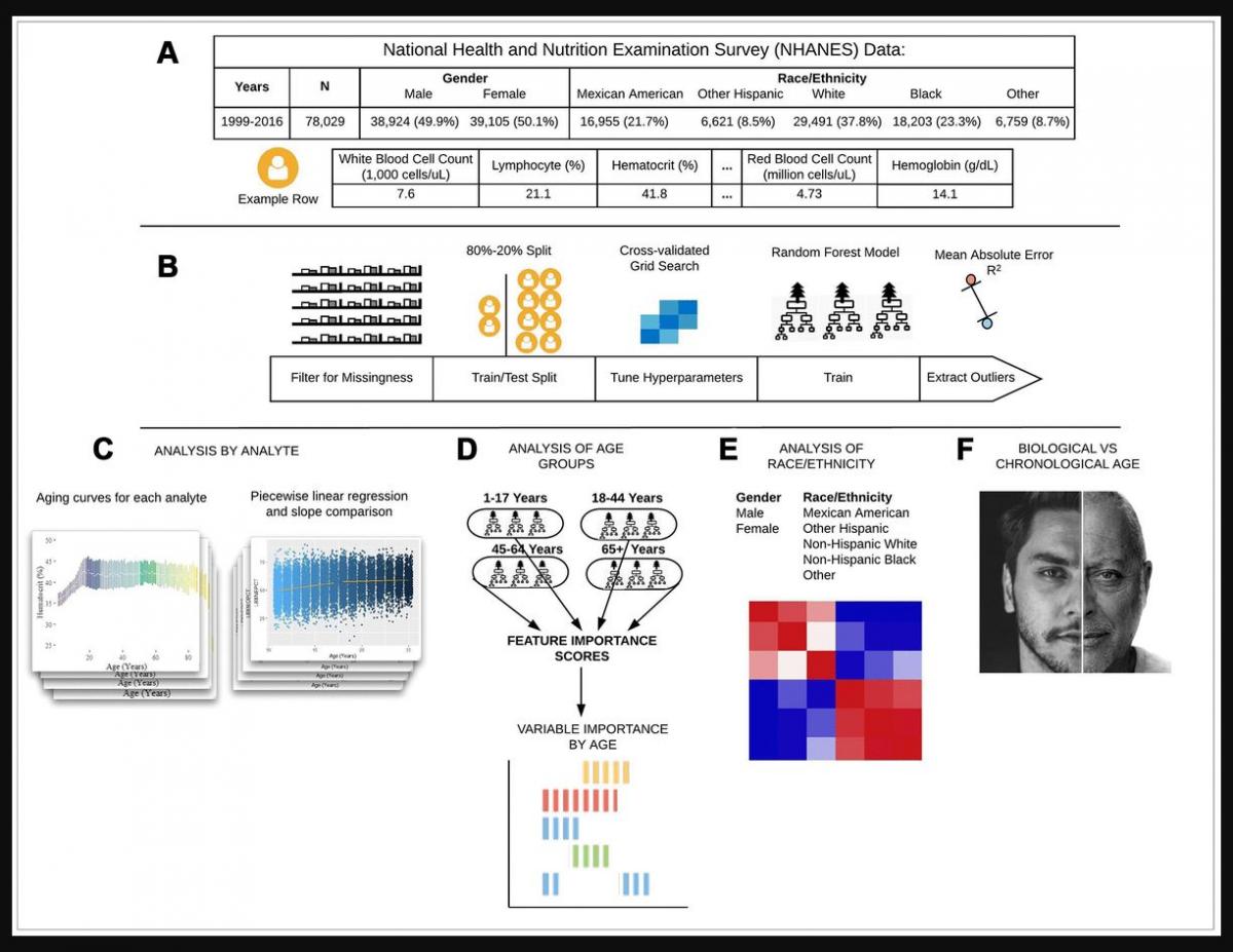
Figure 1. Schematic overview of our study. (A) The CDC NHANES datasets from 1999-2016 (N refers to size before filtering) were used in our analyses; shown are summary statistics and an example row for a single individual in the dataset. (B) An overview of the machine learning pipeline used in the study. We filtered on a set missingness criteria (Methods) and then separated individuals into an 80/20 train/test split. We used a random forest model with hyperparameters tuned using a cross-validated grid search. After training the model we tested using cross-validation and the 20% held-out test set and analyzed outliers. © Aging curves for individual analytes were computed and analyzed for linear and non-linear trends. Piecewise regression analysis and breakpoint estimation were used to estimate breakpoints and compare slopes separated by breakpoints. (D) Models were trained separately for four U.S. Census age groups and feature importance scores were computed for each age group. (E) Models were trained on subgroups of the dataset separated by race and gender. The feature importance scores were calculated for each model and compared across race/gender groups. (F) Analyses of the trajectories of analytes across age ranges were used to compare chronological vs. biological definitions of age.
We also trained separate random forest models for the four main United States Census [22] age groups: [1,18), [18,45), [45,65), 65+. The predictive accuracy of the models differed substantially across age groups (pairwise R2 comparisons were significant while adjusting for multiple comparisons; Methods) (Figure 2; Table 1). The model for the [1,18) age group had the Random forest models were trained on data from individuals across different age ranges within the dataset. Mean absolute error and R-squared are shown in the table as measurements of model performance on held-out data.
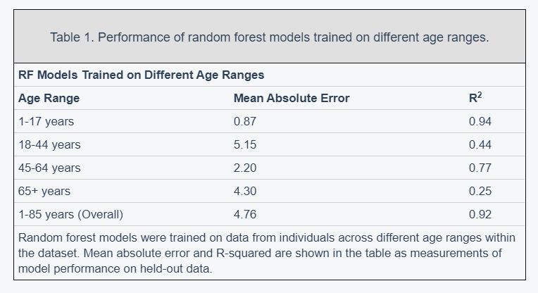
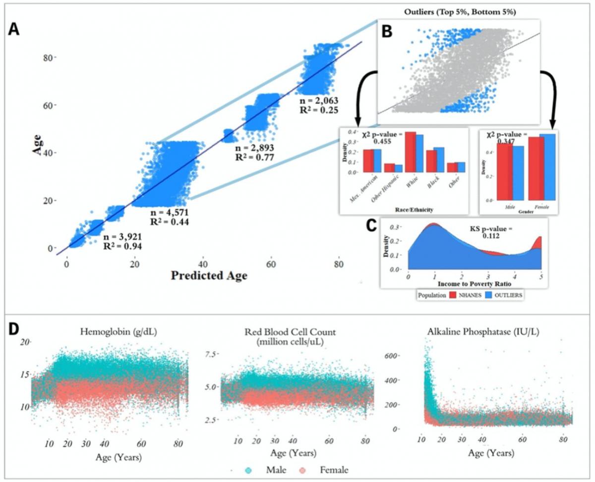
Figure 2. Performance of prediction model across age groups. (A) Actual age vs. predicted age from the random forest model with R2 and sample size (n) for each age range in the test set. (B) Observations with a residual error falling in the top 5% or bottom 5% were identified and compared to the overall NHANES population. © Gender, race, and income to poverty ratio distributions were compared between outliers and the overall NHANES population. (D) Analyte levels by age, colored by gender. Hemoglobin, red blood cell count, and alkaline phosphatase were selected to represent contrasting patterns in the separability of males and females at different age ranges.
most accurate predictions of the four and the model trained on the 65+ age group had the least accurate predictions of the four, as measured by R2 for age prediction in years. In the held-out dataset, the MAE for [1,18) was 0.87 years and the R2 was 0.94. For [18,45), the MAE in the held-out dataset was 5.15 years and the R2 value was 0.44; for [45,65), the MAE was 2.20 years and R2 value was 0.77; for the 65+ cohort, the MAE was 4.30 years and the R2 value was 0.25 (Figure 2).
Feature importance differs substantially across age groups
In order to estimate the predictive power of specific laboratory analytes in a comparable manner, we computed variable importance scores (calculated using the decrease in node impurity using the Gini impurity measure; Methods) for each of the age-specific models across the 356 laboratory analytes. We define the Top-10 set for each age bin as the 10 laboratory analytes with largest variable importance scores for the random forest model trained on that age group, denoted e.g. Top-10[1,18) for the [1,18) age group (similarly for Top-5). We computed relative variable importance scores for each analyte for each age range, and the total relative importance of the Top-5 and Top-10 sets for each age group, denoted e.g. |Top-10[1,18)| for the [1,18) age range.
The analytes in the Top-5 differed substantially across age ranges (Figure 3). The only analyte that appears in the Top-5 for multiple age groups is alanine aminotransferase, which appears in both the [1,18) and 65+ groups. |Top-10[1,18)| was 0.751, |Top-10[18,45)| was 0.294; |Top-10[45,65)| was 0.542; |Top-1065+| was 0.225. |Top-5[1,18)| was 0.567; |Top-5[18,45)| was 0.169; |Top-5[45,65)| was 0.464; |Top-565+| was 0.144 (Supplementary Table 1). Top-5[1,18) consisted of hepatitis B, alkaline phosphatase, lactate dehydrogenase, aspartate aminotransferase, and alanine aminotransferase; Top-5[18,45) consisted of total cholesterol, serum vitamin E, serum cholesterol, glycohemoglobin, and hepatitis B antibody; Top-5[45,65) consisted of herpes simplex 1, herpes simplex 2, toxoplasma, HIV 1,2 combo test, and varicella. Top-565+ consisted of alanine aminotransferase, blood urea nitrogen, lymphocyte percentage, creatinine, and homocysteine (Figure 3).
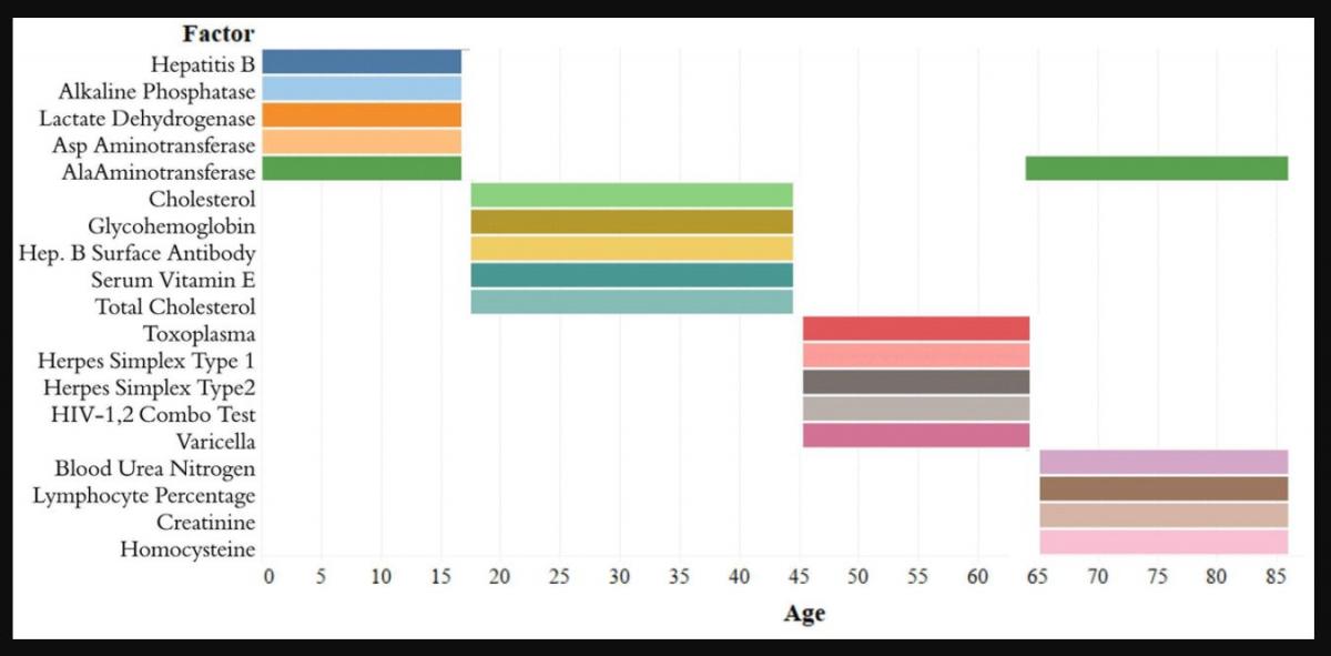
Figure 3. Top-5 variables (based on feature importance score) across age bins. The Top-5 variables based on feature importance scores across the four age groups ([1,18), [18,45), [45,65), 65+) are shown. The variables are different for each age group except for alanine aminotransferase, which is present in the top variables of both [1,18) and 65+ age groups.
Chronological vs. biological age in laboratory data
In the held-out datasets (total n = 13,513), we defined ‘outliers’ as individuals with residual errors in the top 5% or bottom 5% of their age group, representing approximately 37.1 million individuals in the US (based on NHANES sample weights). For the bottom 5% of each age group, the model underestimated their age by an average of 2.20 years (sd = 0.50) for [1,18); 10.9 years (sd = 1.64) for [18,45); 6.38 years (sd = 1.80) for [45,65); and 8.64 years (sd = 1.09) for 65+. For the top 5% of each age group, the model overestimated the age of outliers by an average of 2.47 years (sd = 0.89) for [1,18); 12.23 years (sd = 1.91) for [18,45); 5.52 years (sd = 0.72) for [45,65); and 9.07 years (sd = 1.04) for 65+. We compared the outliers from each age bin with the remaining individuals in the held-out dataset to assess differences in demographic features between these groups (Figure 2). After correcting for multiple comparisons, we found no significant differences between the outlier populations from each age bin and the rest of the individuals from that age bin in gender, race, and income to poverty ratio distributions.
In order to investigate aging in males and females, we stratified 356 analytes individually by age and gender (Figure 2D, Supplementary Figure 2). We found that several analytes, including major blood labs such as red blood cell count, hemoglobin, and hematocrit, and other labs such as alkaline phosphatase, lactate dehydrogenase, and calcium, showed age-related changes that differed starkly between males and females. For hematocrit, hemoglobin, and red blood cell count, male and female values are homogeneously mixed in younger children, separate in the teenage years until male and female values exhibit different ranges, and then cross over again in the senior years. For alkaline phosphatase, this trend is reversed, and sexual dimorphism is apparent in children below 15 years old, and then gradually reduces with age.